. 2020 Apr 9;20(4):10.
doi: 10.1167/jov.20.4.10.

Space of preattentive shape features

Affiliations

Space of preattentive shape features

Liqiang Huang. J Vis. .

Abstract

Four decades of studies in visual attention and visual working memory used visual features such as colors, orientations, and shapes. The layout of their featural space is clearly established for most features (e.g., CIE-Lab for colors) but not shapes. Here, I attempted to reveal the basic dimensions of preattentive shape features by studying how shapes can be positioned relative to one another in a way that matches their perceived similarities. Specifically, 14 shapes were optimized as n-dimensional vectors to achieve the highest linear correlation (r) between the log-distances between C (14, 2) = 91 pairs of shapes and the discriminabilities (d') of these 91 pairs in a texture segregation task. These d' values were measured on a large sample (N = 200) and achieved high reliability (Cronbach's α = 0.982). A vast majority of variances in the results (r = 0.974) can be explained by a three-dimensional SCI shape space: segmentability, compactness, and spikiness.


Figures
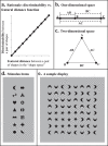
Figure 1.
Figure 1.
Rationale and method. The rationale of this study is illustrated (a). If shapes are represented by vectors in n-dimensional uniform shape space, then there should be a linear discriminability-featural distance relationship: The more discriminable two shapes are from each other, the further away they are from each other in the shape space. Next, the number of dimensions of the shape space can be determined as the minimum number of dimensions required to explain a major portion of the variance in discriminabilities between all the possible pairs of shapes among this set. For example, if we study three shapes, A, B, and C, and measure the three discriminabilities between the three pairs of shapes, we may find the values of dAC, dAB, and dBC can be adequately explained by placing these three shapes in a one-dimensional space (b); alternatively, we may find that all three discriminabilities are roughly equal to each other, and so they therefore have to be explained by placing these three shapes in a two-dimensional space (c). The present study included 14 typical shapes (d). In each trial, a target shape and a background shape were chosen from these 14 shapes and respectively used to generate a rectangular target-shape array inside a background array. Observers were asked to judge, in a very brief (100 ms) and masked display, whether the rectangle was vertical or horizontal (e).
Figure 2.
Figure 2.
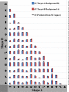
Data. For a pair of shape (A and B), the blue bar represents the d′ of performing a texture segregation task for the Target-A-Background-B condition, whereas the red bar represents the Target-B-Background-A condition. The black line represents the predicted d′ from the SCI shape space. See text for details.
Figure 3.
Figure 3.
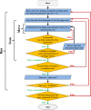
The program flowchart of the optimization algorithm. The present study adopted a general-purpose straightforward algorithm: dimension-by-dimension fixed-step-size movements, implemented as a four-level loop. Here, 14 vectors were used to represent the coordinates of the 14 shape items in the shape space. On the level of whole optimization procedure, multiple runs were started from different sets of random starting vectors and the runs repeated until a best-fitting r had been replicated 20 times. On the level of a run, at the beginning of each run, the step size was set as 0.5. A run consisted of multiple scans. These scans were repeated until meeting the criterion of successfully reaching a maximum of the fitting index r (step size < 0.000001) or until meeting some criteria of terminating a run. On the level of a scan, in each scan, the program sequentially scanned through all dimensions of all vectors. If, in a complete scan, there was no change for any of the dimensions of any of the 14 vectors because the fitting index (r) was already at a maximum, then the step size was halved at the end of this scan. On the level of a move, at this most elementary level, a dimension of a vector attempted to move by the specified step size until the fitting index (r) had reached a maximum. After each movement, the scale of vectors was standardized.
Figure 4.
Figure 4.
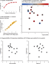
Results and analysis. For number of dimensions = 1 to 6, I used an optimization algorithm to determine the best model (i.e., highest correlation). It seems that the shape space is most reasonably characterized by three dimensions because the fitting is already very good (r = 0.974) and improves relatively little for the subsequent dimensions (a). Following the rationale illustrated in Figure 1a, there is a strong correlation between the log-distances between the 91 pairs of shapes in this 3D shape space and the 91 discriminabilities (d′) between them (b). The best-fitting coordinates of the 14 shapes as 3D vectors were plotted in (c) (and also in (d) that plotted the same data in two graphs). The first dimension (x-axis of (c) and also x-axis of the left graph of (d)) matches well with the conceptual dimension of “segmentability” (e.g., ✚ vs. ●). The second dimension (y-axis of (c) and also y-axis of both graphs of (d)) matches well with the conceptual dimension of “compactness” (e.g., О vs. ▲). The third dimension (hue of bubbles of (c) and also x-axis of the right graph of (d)) matches well with the conceptual dimension of “spikiness” (e.g., formula image vs. ●). Together, they constitute a (s)egmentability-(c)ompactness-sp(i)kiness (SCI) space.
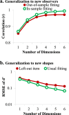
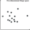
Figure 5.
Figure 5.
Assessments of overfitting. The central problem of overfitting is the failure of making good predictions for new data. For generalization to a new group of observers (a), I used an out-of-sample fitting procedure to assess this problem. Unsurprisingly, the in-sample fitting was better than the out-of-sample fitting, and the difference grew with more dimensions. However, it is also clear that the difference was relatively trivial (r = 0.972 vs. 0.957 for the 3D model), and this suggests that the SCI shape space can be generalized to a new group of observers. For generalization to new shapes (b), I used a leave-one-out fitting procedure to assess this problem. Unsurprisingly, when a shape was left out, the fitting of the shape was worse than the usual fitting, and the difference grew with more dimensions. However, it is also clear that the difference was modest (a 49% increase of RMSE), and this suggests that the SCI shape space can be generalized to new shapes.
Figure 6.
Figure 6.
The best-fitting two-dimensional shape space. It is clearly inadequate and overly compressed. Some of the fundamentally different variations (✚ vs. ● difference; О vs. ● difference) have been forced to reside on almost the same dimension, which is conceptually inappropriate. Therefore, 3D (i.e., SCI) shape space is conceptually better than the two-dimensional shape space.
Figure 7.
Figure 7.
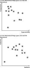
The best-fitting four-dimensional shape space. The layout is rotated so that the first three dimensions approximately match the three dimensions of the SCI shape space. As can be seen in the y-axis of (b), the fourth dimension is not associated with any clear conceptual interpretation. Therefore, 3D (i.e., SCI) shape space is conceptually better than the four-dimensional shape space.
Figure 8.
Figure 8.
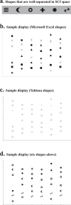
Clearly distinguishable shapes. Shapes are often used as signs and symbols. For these purposes, it is usually desirable to use shapes that are clearly distinguishable from each other. Panel (a) provides a practical guide of 6 shapes that are most well separated in SCI shape space. These shapes are listed in descending order of distinguishability. Therefore, for a set of three clearly distinguishable shapes, the first three should be used, and so forth. Panels (b) and (c) respectively show sample displays in which default symbols of Microsoft Excel and those of Tableau are used, whereas (d) shows one in which these six distinguishable shapes are used. It seems that the series of data can be distinguished more easily from each other in (d) than in (b) and (c).
Figure 9.
Figure 9.
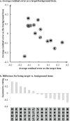
Residual errors. Panel (a) plotted the average residual errors for each shape as the target item and also for each shape as the background item. Panel (b) plotted the difference between being the target and background items. A positive value indicates that the performance tended to be better when a shape was the target shape than was the background shape. The residual errors are clearly affected by the rotational symmetry of a shape, namely, how much a shape looks the same after rotations. For the six shapes with the largest negative differences, four of them are identical for all four orientations (⊞, ✚, ●, and О), whereas for each of the other two shapes (▲ and ★), the four appearances of the four orientations do not appear to be visually very different from each other. On the other hand, for each of the two shapes with the largest positive differences (formula image and formula image), the four (or two) appearances of the different orientations do appear to be very different from each other.

Similar articles

Cited by

References

    1. Anzai A., Peng X., & Van Essen D. C. (2007). Neurons in monkey visual area V2 encode combinations of orientations. Nature Neuroscience, 10, 1313, 10.1038/nn1975. - DOI - PubMed
    1. Bae G. Y., & Flombaum J. I. (2013). Two items remembered as precisely as one how integral features can improve visual working memory. Psychological Science, 24, 2038–2047. - PubMed
    1. Beck J. (1966). Perceptual grouping produced by changes in orientation and shape. Science, 154, 538–540, 10.1126/science.154.3748.538. - DOI - PubMed
    1. Beck J. (1982). Texture segregation. In Beck J. (Ed.), Organization and representation in perception (pp. 285–318). Hillsdale, NJ: Erlbaum.
    1. Biederman I. (1987). Recognition-by-components—a theory of human image understanding. Psychological Review, 94, 115–147, 10.1037/0033-295X.94.2.115. - DOI - PubMed

Publication types