. 2020 Jul 6;21(13):4787.
doi: 10.3390/ijms21134787.

Protein-Protein Interactions Efficiently Modeled by Residue Cluster Classes

Affiliations

Protein-Protein Interactions Efficiently Modeled by Residue Cluster Classes

Albros Hermes Poot Velez et al. Int J Mol Sci. .

Abstract

Predicting protein-protein interactions (PPI) represents an important challenge in structural bioinformatics. Current computational methods display different degrees of accuracy when predicting these interactions. Different factors were proposed to help improve these predictions, including choosing the proper descriptors of proteins to represent these interactions, among others. In the current work, we provide a representative protein structure that is amenable to PPI classification using machine learning approaches, referred to as residue cluster classes. Through sampling and optimization, we identified the best algorithm-parameter pair to classify PPI from more than 360 different training sets. We tested these classifiers against PPI datasets that were not included in the training set but shared sequence similarity with proteins in the training set to reproduce the situation of most proteins sharing sequence similarity with others. We identified a model with almost no PPI error (96-99% of correctly classified instances) and showed that residue cluster classes of protein pairs displayed a distinct pattern between positive and negative protein interactions. Our results indicated that residue cluster classes are structural features relevant to model PPI and provide a novel tool to mathematically model the protein structure/function relationship.

Keywords: machine learning; protein–protein interaction; residue cluster class.


Conflict of interest statement

The authors declare no conflict of interest. The funders had no role in the design of the study, in the collection, analyses, or interpretation of data, in the writing of the manuscript, or in the decision to publish the results.

Figures
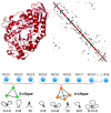
Figure 1
Figure 1
Residue cluster class (RCC) construction. Top panel: The atomic three-dimensional structure of a protein (left) is transformed into a contact map (right) that is used to build the RCC. Lower panel: The RCC is a 26-dimensional vector (RCC1, …, RCC26) derived by grouping residues close together in the three-dimensional space according to a distance criterion. These clusters group three (RCC1-RCC3), four (RCC4-RCC8), five (RCC9-RCC15), and six (RCC16-RCC26) amino acid residues; the image only represents RCC1–RCC8 for brevity. Different clusters of the same size are generated according to their sequence proximity. For instance, a cluster referred to as [1,1,1] represents three residues that are not proximal in the sequence (two or more residues apart) but are proximal to each other in the three-dimensional space.
Figure 2
Figure 2
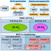
Dataset construction. Top panel: Every PDB reported as positive protein–protein interactions (PPI) in the 3DID database and as negative PPI in the Negatome database were processed to include (sidechain (SC)) or not include (no SC) the atoms of sidechains. A total of 12 different contact maps (contact distances 4–15 Å) were generated for each of these proteins and their residue cluster classes (RCCs) were calculated. Middle panel: The resulting numeric representations for all protein pairs were split into training and testing sets, which did not share the same positive PPI pair but did include the same PFAM domains. The procedure used to separate the positive PPI included in 3DID guaranteed that more instances were included in the training set than the testing set (see Methods). The positive PPI are represented in the figure as [P-P]N in the 3DID, [P-P]a for training, and [P-P]b for testing, where N = a + b and a > b. Due to the limited number of negative cases, we used the same negative set for both training and testing sets. Lower panel: The sum (26 features) or concatenation (52 features) for each RCC in every pair of proteins was obtained. Finally, every PPI numeric representation was normalized, standardized, or kept in its original form (raw).
Figure 3
Figure 3
Distance within and between positive and negative PPI sets. Red circles represent the maximum Euclidian distances between instances of the same class (in this case, negative PPI) and the smallest distances between instances of different classes are shown in black circles. The Y-axis displays the distance values while the X-axis represents the different compared PPI representation compared. The first digit represents the distance used to build the RCCs and the next characters indicate whether the sidechains were included (SC) or not (noSC). Sum or Con indicates if the PPI was represented by the sum or concatenation of the individual RCC of the considered protein pair (see Methods). A red circle below the corresponding black circle indicates the separation of the positive PPI by distance from a negative PPI.
Figure 4
Figure 4
PPI space representation. Based on the distance separation of positive and negative PPI, we envisioned that positive PPI (plus symbols represent instances of positive PPI) would be dispersed over a large region in the space, but close to the negative PPI region(minus symbols represent instances of negative PPI); this proximity is likely the consequence of positive and negative PPI sharing sequence similarity. D represents the diameter of negative PPI, and the distance separating positive and negative PPI sets is represented by d. The red line separating positive and negative PPI sets represents a border that ML methods should be able to identify. The black circle represents k-nearest neighbors.
Figure 5
Figure 5
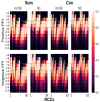
Fraction of RCCs with nonzero values. The graph shows eight different plots presenting the fraction of 26 (sum) or 52 (concatenation) values (X-axis) used to represent PPI (positive PPI) and pairs of proteins that did not interact (negative PPI); fractions are represented by a gradient color, with lighter colors representing those with more nonzero values. On the Y-axis, the distance used to build the contact map is presented (from 4 to 15 Å). The green rectangle indicates the set of distances used to build RCCs, where the number of features (RCC1, RCC2, RCC3, …, RCC26) with values equaling zero was minimum.
Figure 6
Figure 6
Comparison of positive and negative PPI through RCC. The image shows a representative example of the 16 performed comparisons (distance: 7, 8 Å; sidechains: yes, no; PPI RCC construction: sum, concatenation; statistical test: Wilcoxon–Bonferroni, Wilcoxon–Hochberg; all comparisons rendered very similar results (see https://github.com/gdelrioifc/PPI-RCC). The RCCs presented in the figure were obtained using a distance cutoff of 7 Å and included the residue sidechain atoms; the resulting RCCs for each protein pair were added. An asterisk is shown where the distribution of RCC values differs significantly between positive (blue) and negative (orange) PPI sets. The X-axis shows the RCC feature (RCC1, RCC2, …, RCC26) and the Y-axis represents the class of RCC and corresponding compared values. All but one RCC feature (RCC6) rendered a significantly different distribution of RCC values (p < 0.5; Wilcoxon test corrected by Bonferroni criterion).
Figure 7
Figure 7
Sampling of training sets. Upper panel: Two different strategies were followed to deal with over-representation in the training sets, i.e., random elimination of instances from the over-represented positive PPI (under sampling) or generation of instances (synthetic sampling) from the under-represented negative PPI (over sampling). Middle panel: In under sampling, a random sample with equal proportions of positive and negative PPI (1:1), two times more positive than negative PPI (2:1), or three times more positive than negative PPI (3:1) were generated. In over sampling, the 1:1 sample generated in the under sampling, two times more negative than positive (1:2), and three times more negative than positive PPI (1:3) were generated. Lower panel: The RCCs generated for every PPI set were maintained (raw data), standardized, or normalized. The files used for training and testing are available at https://github.com/gdelrioifc/PPI-RCC.
Figure 8
Figure 8
Learning efficiency on sampling training sets with redundancy. The percentages of correctly classified instances (CCI) for the testing sets (X-axis) are plotted against the differences observed in these values for the testing and training (Y-axes) sets. CCI corresponds to true predictions, including both positive and negative PPI. Therefore, 100% on the X-axes corresponds to not failing any prediction on the testing set and a 0 value on the Y-axis corresponds to no difference observed in the prediction between the training and the testing set. The best models are shown in the top right corner. Predictions achieved with raw RCCs are presented as circles, standardized RCCs as squares, and normalized RCCs as triangles. RCCs built using sidechains are otherwise shown in red and black.
Figure 9
Figure 9
Learning efficiency on sampling training sets without redundancy. The percentage of correctly classified instances (CCI) for 360 testing sets (X-axis) is plotted against the difference observed in these values for testing and training (Y-axis). CCI corresponds to true predictions, including both positive and negative PPI. Therefore, 100% on the X-axes corresponds to not failing any prediction on the testing set and a 0 value on the Y-axis corresponds to no difference observed in the prediction between the training and the testing set. The best models are shown the top right corner. RCCs built using sidechains are otherwise represented by red circles or black squares.

Similar articles

References

    1. Carbon S., Douglass E., Dunn N., Good B., Harris N.L., Lewis S.E., Mungall C.J., Basu S., Chisholm R.L., Dodson R.J., et al. The Gene Ontology Resource: 20 years and still GOing strong. Nucleic Acids Res. 2019;47:D330–D338. doi: 10.1093/nar/gky1055. - DOI - PMC - PubMed
    1. Wang J.P., Liu B., Sun Y., Chiang V.L., Sederoff R.R. Enzyme-enzyme interactions in monolignol biosynthesis. Front Plant Sci. 2019;9:1942. doi: 10.3389/fpls.2018.01942. - DOI - PMC - PubMed
    1. Freilich R., Arhar T., Abrams J.L., Gestwicki J.E. Protein-Protein Interactions in the Molecular Chaperone Network. Acc. Chem. Res. 2018;51:940–949. doi: 10.1021/acs.accounts.8b00036. - DOI - PMC - PubMed
    1. Zahiri J., Emamjomeh A., Bagheri S., Ivazeh A., Mahdevar G., Sepasi Tehrani H., Mirzaie M., Fakheri B.A., Mohammad-Noori M. Protein complex prediction: A survey. Genomics. 2020;112:174–183. doi: 10.1016/j.ygeno.2019.01.011. - DOI - PubMed
    1. Liu S., Liu C., Deng L. Machine learning approaches for protein-protein interaction hot spot prediction: Progress and comparative assessment. Molecules. 2018;23:2535. doi: 10.3390/molecules23102535. - DOI - PMC - PubMed

MeSH terms

LinkOut - more resources